All articles published by MDPI are made immediately available worldwide under an open access license. No special
permission is required to reuse all or part of the article published by MDPI, including figures and tables. For
articles published under an open access Creative Common CC BY license, any part of the article may be reused without
permission provided that the original article is clearly cited. For more information, please refer to
https://www.mdpi.com/openaccess.
Feature papers represent the most advanced research with significant potential for high impact in the field. A Feature
Paper should be a substantial original Article that involves several techniques or approaches, provides an outlook for
future research directions and describes possible research applications.
Feature papers are submitted upon individual invitation or recommendation by the scientific editors and must receive
positive feedback from the reviewers.
Editor’s Choice articles are based on recommendations by the scientific editors of MDPI journals from around the world.
Editors select a small number of articles recently published in the journal that they believe will be particularly
interesting to readers, or important in the respective research area. The aim is to provide a snapshot of some of the
most exciting work published in the various research areas of the journal.
Original Submission Date Received: .
You seem to have javascript disabled. Please note that many of the page functionalities won't work as expected without javascript enabled.
The valuation of ecosystem services (ESs) is crucial for preserving ecosystems, assessing natural resources, and making decisions regarding compensation. In this study, we employed the InVEST model’s habitat quality (HQ) module to calculate the HQ and degradation levels in the study area using
[...] Read more.
The valuation of ecosystem services (ESs) is crucial for preserving ecosystems, assessing natural resources, and making decisions regarding compensation. In this study, we employed the InVEST model’s habitat quality (HQ) module to calculate the HQ and degradation levels in the study area using land use/land cover (LULC) data from 2000 to 2020. Our analysis utilized quantitative methods, including spatial correlation, hotspot analysis, and geo-probing, to determine the value of ESs and identify trends. Furthermore, we examined the spatial and temporal variation in the significance of ESs and their driving factors. The results show the following. (1) The primary LULC types in the Zhundong coalfield from 2000 to 2020 are grassland and barren areas. (2) The average value of the HQ index in the study area exhibited a generally decreasing trend. Between 2000 and 2010, HQ significantly declined, particularly in the region’s large barren industrial and mining zones. However, over time, the proportion of sites with minimal degradation improved steadily, resulting in better overall HQ in the study area by 2020. This pertains to the measures put in place by the local government to safeguard and rehabilitate the ecosystem. (3) The spatial distribution of the ecosystem service value (ESV) aligns with changes in HQ and LULC, with significant hotspots primarily observed in forest and grassland areas, nature reserves, and areas around water sources. (4) LULC, temperature, annual precipitation, and elevation are the main drivers of spatial variation in the ESV in the Zhundong area; the spatial variation in the ESV in the Zhundong coalfield is primarily influenced by the interaction between human factors and natural factors, in which LULC plays a dominant role. This study’s findings can guide the development of rational ecological planning, integrating resource conservation mining with effective zoning management.
Full article
There is a huge reservation of loess in the Shanxi mining area in China, which has great potential for preparing supplementary cementitious materials. Loess was modified via mechanical and thermal activation, and the pozzolanic activity was evaluated using an Inductively Coupled Plasma Optical
[...] Read more.
There is a huge reservation of loess in the Shanxi mining area in China, which has great potential for preparing supplementary cementitious materials. Loess was modified via mechanical and thermal activation, and the pozzolanic activity was evaluated using an Inductively Coupled Plasma Optical Emission Spectrometer (ICP-OES). Moreover, the workability of grouting materials prepared using modified loess was assessed. The experimental results revealed that the number of ultrafine particles gradually increased with the grinding time, enhancing the grouting performance. The coordination number of Al decreased upon the breakage of the Al–O–Si bond post-calcination at 400 °C, 550 °C, 700 °C, and 850 °C. Moreover, the breaking of the Si–O covalent bond produced Si-phases, and the pozzolanic activity of loess increased. Furthermore, the modified loess was hydrated with different cement proportions. With increasing grinding time, the overall setting time increased until the longest time of 14.5 h and the fluidity of the slurry decreased until the lowest fluidity of 9.7 cm. However, the fluidity and setting time decreased with increasing calcination temperature. The lowest values were 12.03 cm and 10.05 h. With the increase in pozzolanic activity, more ettringite was produced via hydration, which enhanced the mechanical properties. The maximum strength of the hydrated loess after grinding for 20 min reached 16.5 MPa. The strength of the hydrated loess calcined at 850 °C reached 21 MPa. These experimental findings provide theoretical support for the practical application of loess in grouting.
Full article
Front loaders used in agriculture are characterized by a compact structure, which limits the scope of their application. The loading possibilities are expanded by designing front loaders equipped with telescopic arms. This design increases the loader’s working area, making it easier to load
[...] Read more.
Front loaders used in agriculture are characterized by a compact structure, which limits the scope of their application. The loading possibilities are expanded by designing front loaders equipped with telescopic arms. This design increases the loader’s working area, making it easier to load trucks. It is necessary to work on the arm extension drive and perform strength analyses on the new structures. This article presents a FEM numerical analysis of the structure of an extending front loader and an assessment of the state of stress and the value of displacements under the influence of load. This study discusses the advantages and disadvantages of front loaders compared to telehandlers and the legal requirements and standards for the design of front loaders in Europe. This work presents the concept of loader arm movement and assesses the effectiveness of using hydraulic motors coupled with a screw gear. The obtained results prove that the newly designed extending front loader system is safe and stable.
Full article
Ullazines and their π-expanded derivatives have gained much attention as active components in various applications, such as in organic photovoltaic cells or as photosensitizers for CO2 photoreduction. Here, we report the divergent synthesis of functionalized diazaullazines by means of two different domino-reactions
[...] Read more.
Ullazines and their π-expanded derivatives have gained much attention as active components in various applications, such as in organic photovoltaic cells or as photosensitizers for CO2 photoreduction. Here, we report the divergent synthesis of functionalized diazaullazines by means of two different domino-reactions consisting of either a Povarov/cycloisomerization or alkyne–carbonyl metathesis/cycloisomerization protocol. The corresponding quinolino-diazaullazine and benzoyl-diazaullazine derivatives were obtained in moderate to good yields. Their optical and electronic properties were studied and compared to related, literature-known compounds to obtain insights into the impact of nitrogen doping and π-expansion.
Full article
This study is based on the need to improve packaging sustainability in the food industry. Its aim was to assess the performance of a recyclable plastic material for semi-hard sheep’s cheese wedges packaging as an alternative to conventional non-sustainable plastic materials. Four different
[...] Read more.
This study is based on the need to improve packaging sustainability in the food industry. Its aim was to assess the performance of a recyclable plastic material for semi-hard sheep’s cheese wedges packaging as an alternative to conventional non-sustainable plastic materials. Four different packaging treatments (air, vacuum, and CO2/N2 gas mixtures 50/50 and 80/20% (v/v)) were studied. Changes in gas headspace composition, sensory properties, cheese gross composition, weight loss, pH, colour, and texture profile were investigated at 5 ± 1 °C storage for 56 days. The sensory analysis indicated that vacuum packaging scored the worst in paste appearance and holes, and air atmosphere the worst in flavour; it was concluded that cheeses were unfit from day 14–21 onwards. Air and vacuum packaging were responsible for most of the significant changes identified in the texture profile analysis, and most of these happened in the early stages of storage. The colour parameters a* and b* differentiated the air packaging from the rest of the conditions. As in previous studies using conventional plastic materials, modified atmosphere packaging, either CO2/N2 50/50 or 80/20% (v/v), was the most effective preserving technique to ensure the quality of this type of cheese when comparing air and vacuum packaging treatments.
Full article
Fresh aquatic products, due to their high water activity, are susceptible to microbial contamination and spoilage, resulting in a short shelf life. Drying is a commonly used method to extend the shelf life of these products by reducing the moisture content, inhibiting microbial
[...] Read more.
Fresh aquatic products, due to their high water activity, are susceptible to microbial contamination and spoilage, resulting in a short shelf life. Drying is a commonly used method to extend the shelf life of these products by reducing the moisture content, inhibiting microbial growth, and slowing down enzymatic and chemical reactions. However, the drying process of aquatic products involves chemical reactions such as oxidation and hydrolysis, which pose challenges in obtaining high-quality dried products. This paper provides a comprehensive review of drying processing techniques for aquatic products, including drying preprocessing, drying technologies, and non-destructive monitoring techniques, and discusses their advantages and challenges. Furthermore, the impact of the drying process on the quality attributes of dried products, including sensory quality, nutritional components, and microbial aspects, is analyzed. Finally, the challenges faced by drying processing techniques for aquatic products are identified, and future research prospects are outlined, aiming to further advance research and innovation in this field.
Full article
Prior studies into fatigue crack growth (FCG) in fibre-reinforced polymer composites have shown that the two methodologies of Simple-Scaling and the Hartman–Schijve crack growth equation, which is based on relating the FCG rate to the Schwalbe crack driving force, Δκ, were
[...] Read more.
Prior studies into fatigue crack growth (FCG) in fibre-reinforced polymer composites have shown that the two methodologies of Simple-Scaling and the Hartman–Schijve crack growth equation, which is based on relating the FCG rate to the Schwalbe crack driving force, Δκ, were able to account for differences observed in the measured delamination growth curves. The present paper reveals that these two approaches are also able to account for differences seen in plots of the rate of crack growth, da/dt, versus the range of the imposed stress intensity factor, ΔK, associated with fatigue tests on different grades ofhigh-density polyethylene (HDPE) polymers, before and after electron-beam irradiation, and for tests conducted at different R ratios. Also, these studies are successfully extended to consider FCG in an acrylonitrile butadiene styrene (ABS) polymer that is processed using both conventional injection moulding and additive-manufactured (AM) 3D printing.
Full article
For hybrid direct sequence/frequency hopping (DS/FH) spread spectrum signals, even if the relative motion speed between the transmitter and receiver remains constant, the Doppler frequency will vary due to the continuous hopping of the carrier frequency. Under high dynamic conditions, the first-order and
[...] Read more.
For hybrid direct sequence/frequency hopping (DS/FH) spread spectrum signals, even if the relative motion speed between the transmitter and receiver remains constant, the Doppler frequency will vary due to the continuous hopping of the carrier frequency. Under high dynamic conditions, the first-order and second-order change rates of the Doppler frequency attached to the received signal further increase the Doppler frequency agility, making it difficult for the carrier tracking loop to maintain steady-state tracking. To address these issues, a high dynamic velocity locked loop (HD-VLL) is proposed in this paper. Specifically, the accumulated phase tracking error caused by acceleration and jerk is first analyzed. Subsequently, to compensate for this phase tracking error with the system clock, the proposed loop adds an acceleration compensation module and a jerk compensation module. However, this results in the output of the high dynamic loop filter being updated with the system clock, which contradicts the multiplexing design of a traditional loop filter for parallel signal processing, making the hardware implementation of an HD-VLL impractical. Therefore, this contradiction leads us to design an HD-VLL-based multi-carrier NCO (HD-VLL-NCO). The HD-VLL and HD-VLL-NCO are simulated, revealing the HD-VLL’s superior dynamic adaptability and steady-state tracking, while the HD-VLL-NCO achieves comparable accuracy with the appropriate truncation bit width.
Full article
Cutaneous leishmaniasis (CL) is a zoonotic disease, manifested as chronic ulcers, potentially leaving unattractive scars. There is no preventive vaccination or optimal medication against leishmaniasis. Chemotherapy generally depends upon a small group of compounds, each with its own efficacy, toxicity, and rate of
[...] Read more.
Cutaneous leishmaniasis (CL) is a zoonotic disease, manifested as chronic ulcers, potentially leaving unattractive scars. There is no preventive vaccination or optimal medication against leishmaniasis. Chemotherapy generally depends upon a small group of compounds, each with its own efficacy, toxicity, and rate of drug resistance. To date, no standardized, simple, safe, and highly effective regimen for treating CL exists. Therefore, there is an urgent need to develop new optimal medication for this disease. Sesquiterpen thio-alkaloids constitute a group of plant secondary metabolites that bear great potential for medicinal uses. The nupharidines found in Nuphar lutea belong to this group of compounds. We have previously published that Nuphar lutea semi-purified extract containing major components of nupharidines has strong anti-leishmanial activity in vitro. Here, we present in vivo data on the therapeutic benefit of the extract against Leishmania major (L. major) in infected mice. We also expanded these observations by establishing the therapeutic effect of the extract-purified nupharidine 6,6′-dihydroxythiobinupharidine (DTBN) in vitro against promastigotes and intracellular amastigotes as well as in vivo in L. major-infected mice. The results suggest that this novel anti-parasitic small molecule has the potential to be further developed against Leishmania.Full article
Alterations in a mother’s metabolism and endocrine system, due to unbalanced nutrition, may increase the risk of both metabolic and non-metabolic disorders in the offspring’s childhood and adulthood. The risk of obesity in the offspring can be determined by the interplay between maternal
[...] Read more.
Alterations in a mother’s metabolism and endocrine system, due to unbalanced nutrition, may increase the risk of both metabolic and non-metabolic disorders in the offspring’s childhood and adulthood. The risk of obesity in the offspring can be determined by the interplay between maternal nutrition and lifestyle, intrauterine environment, epigenetic modifications, and early postnatal factors. Several studies have indicated that the fetal bowel begins to colonize before birth and that, during birth and nursing, the gut microbiota continues to change. The mother’s gut microbiota is primarily transferred to the fetus through maternal nutrition and the environment. In this way, it is able to impact the establishment of the early fetal and neonatal microbiome, resulting in epigenetic signatures that can possibly predispose the offspring to the development of obesity in later life. However, antioxidants and exercise in the mother have been shown to improve the offspring’s metabolism, with improvements in leptin, triglycerides, adiponectin, and insulin resistance, as well as in the fetal birth weight through epigenetic mechanisms. Therefore, in this extensive literature review, we aimed to investigate the relationship between maternal diet, epigenetics, and gut microbiota in order to expand on current knowledge and identify novel potential preventative strategies for lowering the risk of obesity in children and adults.
Full article
Rice (Oryza sativa) is one of the most important staple foods worldwide. However, rice blast disease, caused by the ascomycete fungus Magnaporthe oryzae, seriously affects the yield and quality of rice. Calmodulin-binding transcriptional activators (CAMTAs) play vital roles in the
[...] Read more.
Rice (Oryza sativa) is one of the most important staple foods worldwide. However, rice blast disease, caused by the ascomycete fungus Magnaporthe oryzae, seriously affects the yield and quality of rice. Calmodulin-binding transcriptional activators (CAMTAs) play vital roles in the response to biotic stresses. In this study, we showed that OsCAMTA3 and CAMTA PROTEIN LIKE (OsCAMTAPL), an OsCAMTA3 homolog that lacks the DNA-binding domain, functioned together in negatively regulating disease resistance in rice. OsCAMTA3 associated with OsCAMTAPL. The oscamta3 and oscamtapl mutants showed enhanced resistance compared to wild-type plants, and oscamta3/pl double mutants showed more robust resistance to M. oryzae than oscamta3 or oscamtapl. An RNA-Seq analysis revealed that 59 and 73 genes, respectively, were differentially expressed in wild-type plants and oscamta3 before and after inoculation with M. oryzae, including OsALDH2B1, an acetaldehyde dehydrogenase that negatively regulates plant immunity. OsCAMTA3 could directly bind to the promoter of OsALDH2B1, and OsALDH2B1 expression was decreased in oscamta3, oscamtapl, and oscamta3/pl mutants. In conclusion, OsCAMTA3 associates with OsCAMTAPL to regulate disease resistance by binding and activating the expression of OsALDH2B1 in rice, which reveals a strategy by which rice controls rice blast disease and provides important genes for resistance breeding holding a certain positive impact on ensuring food security.
Full article
Epigenetic alterations my play a role in the aggressive behavior of Non-Small Cell Lung Cancer (NSCLC). Treatment with the histone deacetylase inhibitor suberoylanilide hydroxamic acid (SAHA, vorinostat) has been reported to interfere with the proliferative and invasive potential of NSCLC cells. In addition,
[...] Read more.
Epigenetic alterations my play a role in the aggressive behavior of Non-Small Cell Lung Cancer (NSCLC). Treatment with the histone deacetylase inhibitor suberoylanilide hydroxamic acid (SAHA, vorinostat) has been reported to interfere with the proliferative and invasive potential of NSCLC cells. In addition, the DNA methyltransferase inhibitor azacytidine (AZA, vidaza) can modulate the levels of the metastasis suppressor KiSS-1. Thus, since cisplatin is still clinically available for NSCLC therapy, the aim of this study was to evaluate drug combinations between cisplatin and SAHA as well as AZA using cisplatin-sensitive H460 and -resistant H460/Pt NSCLC cells in relation to KiSS-1 modulation. An analysis of drug interaction according to the Combination-Index values indicated a more marked synergistic effect when the exposure to SAHA or AZA preceded cisplatin treatment with respect to a simultaneous schedule. A modulation of proteins involved in apoptosis (p53, Bax) was found in both sensitive and resistant cells, and compared to the treatment with epigenetic agents alone, the combination of cisplatin and SAHA or AZA increased apoptosis induction. The epigenetic treatments, both as single agents and in combination, increased the release of KiSS-1. Finally, the exposure of cisplatin-sensitive and -resistant cells to the kisspeptin KP10 enhanced cisplatin induced cell death. The efficacy of the combination of SAHA and cisplatin was tested in vivo after subcutaneous inoculum of parental and resistant cells in immunodeficient mice. A significant tumor volume inhibition was found when mice bearing advanced tumors were treated with the combination of SAHA and cisplatin according to the best schedule identified in cellular studies. These results, together with the available literature, support that epigenetic drugs are amenable for the combination treatment of NSCLC, including patients bearing cisplatin-resistant tumors.
Full article
Protein posttranslational modifications are important factors that mediate the fine regulation of signaling molecules. O-linked β-N-acetylglucosamine-modification (O-GlcNAcylation) is a monosaccharide modification on N-acetylglucosamine linked to the hydroxyl terminus of serine and threonine of proteins. O-GlcNAcylation is responsive to cellular stress as a reversible
[...] Read more.
Protein posttranslational modifications are important factors that mediate the fine regulation of signaling molecules. O-linked β-N-acetylglucosamine-modification (O-GlcNAcylation) is a monosaccharide modification on N-acetylglucosamine linked to the hydroxyl terminus of serine and threonine of proteins. O-GlcNAcylation is responsive to cellular stress as a reversible and posttranslational modification of nuclear, mitochondrial and cytoplasmic proteins. Mitochondrial proteins are the main targets of O-GlcNAcylation and O-GlcNAcylation is a key regulator of mitochondrial homeostasis by directly regulating the mitochondrial proteome or protein activity and function. Disruption of O-GlcNAcylation is closely related to mitochondrial dysfunction. More importantly, the O-GlcNAcylation of cardiac proteins has been proven to be protective or harmful to cardiac function. Mitochondrial homeostasis is crucial for cardiac contractile function and myocardial cell metabolism, and the imbalance of mitochondrial homeostasis plays a crucial role in the pathogenesis of cardiovascular diseases (CVDs). In this review, we will focus on the interactions between protein O-GlcNAcylation and mitochondrial homeostasis and provide insights on the role of mitochondrial protein O-GlcNAcylation in CVDs.
Full article
This research confronts the persistent challenge of data scarcity in medical machine learning by introducing a pioneering methodology that harnesses the capabilities of Generative Pre-trained Transformers (GPT). In response to the limitations posed by a dearth of labeled medical data, our approach involves
[...] Read more.
This research confronts the persistent challenge of data scarcity in medical machine learning by introducing a pioneering methodology that harnesses the capabilities of Generative Pre-trained Transformers (GPT). In response to the limitations posed by a dearth of labeled medical data, our approach involves the synthetic generation of comprehensive patient discharge messages, setting a new standard in the field with GPT autonomously generating 20 fields. Through a meticulous review of the existing literature, we systematically explore GPT’s aptitude for synthetic data generation and feature extraction, providing a robust foundation for subsequent phases of the research. The empirical demonstration showcases the transformative potential of our proposed solution, presenting over 70 patient discharge messages with synthetically generated fields, including severity and chances of hospital re-admission with justification. Moreover, the data had been deployed in a mobile solution where regression algorithms autonomously identified the correlated factors for ascertaining the severity of patients’ conditions. This study not only establishes a novel and comprehensive methodology but also contributes significantly to medical machine learning, presenting the most extensive patient discharge summaries reported in the literature. The results underscore the efficacy of GPT in overcoming data scarcity challenges and pave the way for future research to refine and expand the application of GPT in diverse medical contexts.
Full article
Given the aging global population, identifying heart failure (HF) phenotypes has become crucial, as distinct disease characteristics can influence treatment and prognosis in older adults. This study aimed to analyze the association between clustering of cardiovascular risk factors and HF in older adults.
[...] Read more.
Given the aging global population, identifying heart failure (HF) phenotypes has become crucial, as distinct disease characteristics can influence treatment and prognosis in older adults. This study aimed to analyze the association between clustering of cardiovascular risk factors and HF in older adults. A cross-sectional epidemiological study was conducted with 1322 older adults (55% women, mean age 70.4) seen in primary health care. Diagnosis of HF was performed by a cardiologist based on diagnostic tests and medical history. Cardiovascular risk factors included hypertension, diabetes, hypercholesterolemia, and smoking. Using logistic regression, potential associations were tested. Individual risk factor analysis showed that older adults with hypertension, diabetes, or hypercholesterolemia had up to 7.6 times higher odds to have HF. The cluster where older adults had only one risk factor instead of none increased the odds of HF by 53.0%. Additionally, the odds of older patients having HF ranged from 3.59 times for the two-risk factor cluster to 20.61 times for the simultaneous presence of all four factors. The analysis of clusters substantially increasing HF risk in older adults revealed the importance of individualizing subgroups with distinct HF pathophysiologies. The clinical significance of these clusters can be beneficial in guiding a more personalized therapeutic approach.
Full article
Ultrasonic wireless power transfer technology (UWPT) represents a key technology employed for energizing implantable medical devices (IMDs). In recent years, aluminum nitride (AlN) has gained significant attention due to its biocompatibility and compatibility with complementary metal-oxide-semiconductor (CMOS) technology. In the meantime, the integration
[...] Read more.
Ultrasonic wireless power transfer technology (UWPT) represents a key technology employed for energizing implantable medical devices (IMDs). In recent years, aluminum nitride (AlN) has gained significant attention due to its biocompatibility and compatibility with complementary metal-oxide-semiconductor (CMOS) technology. In the meantime, the integration of scandium-doped aluminum nitride (Al90.4%Sc9.6%N) is an effective solution to address the sensitivity limitations of AlN material for both receiving and transmission capabilities. This study focuses on developing a miniaturized UWPT receiver device based on AlScN piezoelectric micro-electromechanical transducers (PMUTs). The proposed receiver features a PMUT array of 2.8 × 2.8 mm2 comprising 13 × 13 square elements. An acoustic matching gel is applied to address acoustic impedance mismatch when operating in liquid environments. Experimental evaluations in deionized water demonstrated that the power transfer efficiency (PTE) is up to 2.33%. The back-end signal processing circuitry includes voltage-doubling rectification, energy storage, and voltage regulation conversion sections, which effectively transform the generated AC signal into a stable 3.3 V DC voltage output and successfully light a commercial LED. This research extends the scope of wireless charging applications and paves the way for further device miniaturization by integrating all system components into a single chip in future implementations.
Full article
Osteoporosis, characterized by reduced bone density and increased fracture risk, affects over 200 million people worldwide, predominantly older adults and postmenopausal women. The disruption of the balance between bone-forming osteoblasts and bone-resorbing osteoclasts underlies osteoporosis pathophysiology. Standard treatment includes lifestyle modifications, calcium and
[...] Read more.
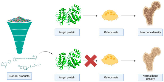
Osteoporosis, characterized by reduced bone density and increased fracture risk, affects over 200 million people worldwide, predominantly older adults and postmenopausal women. The disruption of the balance between bone-forming osteoblasts and bone-resorbing osteoclasts underlies osteoporosis pathophysiology. Standard treatment includes lifestyle modifications, calcium and vitamin D supplementation and specific drugs that either inhibit osteoclasts or stimulate osteoblasts. However, these treatments have limitations, including side effects and compliance issues. Natural products have emerged as potential osteoporosis therapeutics, but their mechanisms of action remain poorly understood. In this study, we investigate the efficacy of natural compounds in modulating molecular targets relevant to osteoporosis, focusing on the Mitogen-Activated Protein Kinase (MAPK) pathway and the gut microbiome’s influence on bone homeostasis. Using an in silico and in vitro methodology, we have identified quercetin as a promising candidate in modulating MAPK activity, offering a potential therapeutic perspective for osteoporosis treatment.
Full article
Although research has shown that moral distress harms mental health in diverse populations, information on potential moderators of such associations is scarce. In a sample of sub-Saharan African nurses, we examined the link between moral distress and depressive symptoms. We explored for whom
[...] Read more.
Although research has shown that moral distress harms mental health in diverse populations, information on potential moderators of such associations is scarce. In a sample of sub-Saharan African nurses, we examined the link between moral distress and depressive symptoms. We explored for whom and when such relationships may hold with regard to gender, age, and work experience. Participants consisted of 398 nurses drawn from a tertiary healthcare institution in southeastern Nigeria. Data were collected using the Moral Distress Questionnaire (MDQ) for clinical nurses, and the Center for Epidemiological Studies Depression Scale Revised (CEDS-R). Hayes regression-based macro results for the moderation effects indicated that the association of high moral distress with increased depressive symptoms was robust for women but not significant for men. Although older age and higher years of nursing experience were associated with reduced symptoms of depression, nurses’ age and years of work experience did not moderate the relationship between moral distress and depressive symptoms. To promote mental well-being and preserve the integrity of nurses, gender-based differentials in how morals contribute depressive symptoms should be considered in policy and practice.
Full article
Multiple natural frequencies may be encountered when analyzing the essential natural vibration of a symmetric mechanical system or sub-structure system or a system with special parameters. The transfer matrix method (TMM) is a useful tool for analyzing the natural vibration characteristics of mechanical
[...] Read more.
Multiple natural frequencies may be encountered when analyzing the essential natural vibration of a symmetric mechanical system or sub-structure system or a system with special parameters. The transfer matrix method (TMM) is a useful tool for analyzing the natural vibration characteristics of mechanical or structural systems. It derives a nonlinear eigen-problem (NEP) in general, even a transcendental eigen-problem. This investigation addresses the NEP in TMM and proposes a novel method, called the determinant-differentiation-based method, for calculating multiple natural frequencies and determining their multiplicities. Firstly, the characteristic determinant is differentiated with respect to frequency, transforming the even multiple natural frequencies into the odd multiple zeros of the differentiation of the characteristic determinant. The odd multiple zeros of the first derivative of the characteristic determinant and the odd multiple natural frequencies can be obtained using the bisection method. Among the odd multiple zeros, the even multiple natural frequencies are picked out by the proposed judgment criteria. Then, the natural frequency multiplicities are determined by the higher-order derivatives of the characteristic determinant. Finally, several numerical simulations including the multiple natural frequencies show that the proposed method can effectively calculate the multiple natural frequencies and determine their multiplicities.
Full article
Mathematical modeling is widely used for describing infection transmission and evaluating interventions. The lack of reliable social parameters in the literature has been mentioned by many modeling studies, leading to limitations in the validity and interpretation of the results. Using data from the
[...] Read more.
Mathematical modeling is widely used for describing infection transmission and evaluating interventions. The lack of reliable social parameters in the literature has been mentioned by many modeling studies, leading to limitations in the validity and interpretation of the results. Using data from the European MSM Internet survey 2017, we developed a network model to describe sex acts among MSM in Belgium. The model simulates daily sex acts among steady, persistent casual and one-off partners in a population of 10,000 MSM, grouped as low- or high-activity by using three different definitions. Model calibration was used to estimate partnership duration and homophily rates to match the distribution of cumulative sex partners over 12 months. We estimated an average duration between 1065 and 1409 days for steady partnerships, 4–6 and 251–299 days for assortative high- and low-activity individuals and 8–13 days for disassortative persistent casual partnerships, respectively, varying across the three definitions. High-quality data on social network and behavioral parameters are scarce in the literature. Our study addresses this lack of information by providing a method to estimate crucial parameters for network specification.
Full article
Background and objectives: while acute ischemic stroke is the leading cause of epilepsy in the elderly population, data about its risk factors have been conflicting. Therefore, the aim of our study is to determine the association of early and late epileptic seizures after
[...] Read more.
Background and objectives: while acute ischemic stroke is the leading cause of epilepsy in the elderly population, data about its risk factors have been conflicting. Therefore, the aim of our study is to determine the association of early and late epileptic seizures after acute ischemic stroke with cerebral cortical involvement and electroencephalographic changes. Materials and methods: a prospective cohort study in the Hospital of the Lithuanian University of Health Sciences Kaunas Clinics Department of Neurology was conducted and enrolled 376 acute ischemic stroke patients. Data about the demographical, clinical, radiological, and encephalographic changes was gathered. Patients were followed for 1 year after stroke and assessed for late ES. Results: the incidence of ES was 4.5%, the incidence of early ES was 2.7% and the incidence of late ES was 2.4%. The occurrence of early ES increased the probability of developing late ES. There was no association between acute cerebral cortical damage and the occurrence of ES, including both early and late ES. However, interictal epileptiform discharges were associated with the occurrence of ES, including both early and late ES.
Full article
Pyridoxal and pyridoxal 5′-phosphate are aldehyde forms of B6 vitamin that can easily be transformed into each other in the living organism. The presence of a phosphate group, however, provides the related compounds (e.g., hydrazones) with better solubility in water. In addition,
[...] Read more.
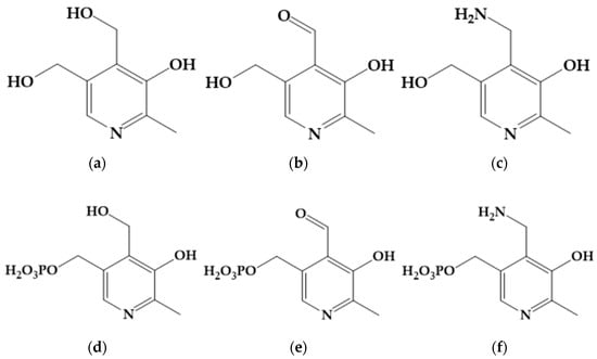
Pyridoxal and pyridoxal 5′-phosphate are aldehyde forms of B6 vitamin that can easily be transformed into each other in the living organism. The presence of a phosphate group, however, provides the related compounds (e.g., hydrazones) with better solubility in water. In addition, the phosphate group may sometimes act as a binding center for metal ions. In particular, a phosphate group can be a strong ligand for a gold(III) ion, which is of interest for researchers for the anti-tumor and antimicrobial potential of gold(III). This paper aims to answer whether the phosphate group is involved in the complex formation between gold(III) and hydrazones derived from pyridoxal 5′-phosphate. The answer is negative, since the comparison of the stability constants determined for the gold(III) complexes with pyridoxal- and pyridoxal 5′-phosphate-derived hydrazones showed a negligible difference. In addition, quantum chemical calculations confirmed that the preferential coordination of two series of phosphorylated and non-phosphorylated hydrazones to gold(III) ion is similar. The preferential protonation modes for the gold(III) complexes were also determined using experimental and calculated data.
Full article
Multi-layer complex structures are widely used in large-scale engineering structures because of their diverse combinations of properties and excellent overall performance. However, multi-layer complex structures are prone to interlaminar debonding damage during use. Therefore, it is necessary to monitor debonding damage in engineering
[...] Read more.
Multi-layer complex structures are widely used in large-scale engineering structures because of their diverse combinations of properties and excellent overall performance. However, multi-layer complex structures are prone to interlaminar debonding damage during use. Therefore, it is necessary to monitor debonding damage in engineering applications to determine structural integrity. In this paper, a damage information extraction method with ladder feature mining for Lamb waves is proposed. The method is able to optimize and screen effective damage information through ladder-type damage extraction. It is suitable for evaluating the severity of debonding damage in aluminum-foamed silicone rubber, a novel multi-layer complex structure. The proposed method contains ladder feature mining stages of damage information selection and damage feature fusion, realizing a multi-level damage information extraction process from coarse to fine. The results show that the accuracy of damage severity assessment by the damage information extraction method with ladder feature mining is improved by more than 5% compared to other methods. The effectiveness and accuracy of the method in assessing the damage severity of multi-layer complex structures are demonstrated, providing a new perspective and solution for damage monitoring of multi-layer complex structures.
Full article